In this section we will address the same problem we did in Section 1.9.1, but we will leave the task of solving the resulting equations to a CLP system. Recall the precedence net in Figure 1.3, and suppose that we want the whole job to be finished in 10 units of time or less. In that example we used finite domain variables, and in this programming example we will use interval variables to simulate FD variables.
Recall that the constraints for the precedence net were
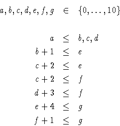
These can be translated into Prolog IV using the following clause:
pn1(A, B, C, D, E, F, G):-
   ge(A, 0),
   le(G, 10),
   ge(B,  A), ge(C, A), ge(D, A),
   ge(E, B .+. 1), ge(E, C .+. 2),
   ge(F, C .+. 2), ge(F, D .+. 3),
   ge(G, E .+. 4), ge(G, F .+. 1).
where variables in the head of the clause correspond to nodes in the graph, and the maximum and minimum starting times for the corresponding job are precisely the bounds of the variables. Time constraints are directly encoded as Prolog IV constraints. After loading this simple program in the system, making a query yields the following result:
?- pn1(A,B,C,D,E,F,G).
   G ~ cc(6,10), F ~ cc(3,9), E ~ cc(2,6), D ~ cc(0,6),
   C ~ cc(0,4), B ~ cc(0,5), A ~ cc(0,4).
The allowed range for each variable represents the slack in the start time for the corresponding task. We can minimize the total time of the project by setting the time of the end task to its lower bound:
?- pn1(A,B,C,D,E,F,G), glb(G, G).
   G = 6, E = 2, C = 0, A = 0,
   F ~ cc(3,5), D ~ cc(0,2), B ~ cc(0,1).
As expected, some variables do not have slack: those are the ones corresponding to critical tasks, whose delay would imply a delay of the whole project.
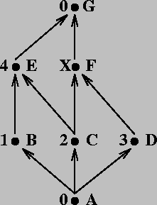
A variant of the project is presented in Figure 3.1. In that figure, there is a task (F) whose duration we can change. Speeding it up will cost more resources, slowing it down will make it cheaper. We want to know what is the minimum resource consumption so that the project is not delayed. We can model this by using the following clause:
pn2(A, B, C, D, E, F, G, X):-
   ge(A, 0), le(G, 10),
   ge(B,  A), ge(C, A), ge(D, A),
   ge(E, B .+. 1), ge(E, C .+. 2),
   ge(F, C .+. 2), ge(F, D .+. 3),
   ge(G, E .+. 4), ge(G, F .+. X).
X, the length of task F, is added to the variables in the head, since we want to access it. A possible query which minimizes project time and maximizes F's duration is:
?- pn2(A, B, C, D, E, F, G, X), glb(G,G), lub(X,X).
   X = 3, G = 6, F = 3, E = 2, D = 0,
   C = 0, A = 0, B ~ cc(0,1).
The last variant of this problem is depicted in Figure 3.2. Two tasks, B and D have a length which is not fixed, but there are some additional constraints which relate their lengths: any of them can be finished in 2 units of time at best, but shared resources disallow finishing both tasks in the minimum time possible: the addition of the duration of both tasks is always 6 units of time.
The constraints which describe the net, again in Prolog IV syntax, are expressed in the following clause:
pn3(A, B, C, D, E, F, G, X, Y):-
   ge(A, 0), le(G, 10),
   ge(X, 2), ge(Y, 2), X .+. Y = 6,
   ge(B,  A), ge(C, A), ge(D, A),
   ge(E, B .+. X), ge(E, C .+. 2),
   ge(F, C .+. 2), ge(F, D .+. Y),
   ge(G, E .+. 4), ge(G, F .+. 1).
The query to ask for a solution, and the answer returned, is as follows:
?- pn3(A,B,C,D,E,F,G,X,Y), glb(G,G).
   Y = 4, X = 2, G = 6, E = 2, C = 0,
   B = 0, A = 0, F ~ cc(4,5), D ~ cc(0,1).
which means that, since X has the minimum possible value, task B is the one to be accelerated. Also, all tasks but F and D are critical now.
The approach we have followed to maximize / minimize a constraint problem is a very naïve one: taking the maximum value of a variable and sticking to it. This does not always work because, since the non-linear solver (as finite domain solvers) is not complete, and there are often values in the range of a variable which are not actually compatible with the problem constraints:
?- X ~ cc(-2, 2), X .*. X  = 1.
   X ~ cc(-2, 2).
The solver did not work out a solution for this quadratic equation (e.g., X = 1 and X = -1), and the initial interval for the variable remains unchanged. If one adds the additional constraint that the solution must be smaller than 1:
?- X ~ cc(-2, 2), X .*. X  = 1, X ~ lt(1).
   X ~ cc(-2,-0.5).
the answer approximates better the solution. But since there is no algorithm for solving non-linear equations, these are left as constraints. The only way to reach a solution to those problems is enumerating, or waiting for variables in the problem to become ground (or, at least, more constrained) so that the solver can decide if the values are compatible with the constraints. For specialized cases (such as maximization or minimization) the solvers include builtin strategies (e.g., branch and bound) which converge to a solution faster than blind enumeration. These strategies are accessible by calling ad-hoc predicates:
?- X ~ cc(-2, 2), X .*. X  = 1, min(X, 0, X), realsplit([X]).
   X = -1.