Trees

We will now turn to a more sophisticated data structure: trees. We will actually only deal with binary trees, because other trees are easily derived. Binary trees are either an empty node, or a node which contains a piece of information, and from which two subtrees are hanging. At the moment we will not suppose any order in the elements of the tree. We will also use trees to exemplify the construction of data structures in CLP languages.

In general, complex data structures are built using functors--much like records are used in C, C++, or Pascal. A significant difference is that there is no need to declare a type, since the structure of the data and the access to their elements is automatically performed by matching and unification. We will use the functor tree/3 as the basic structure for a nonempty node, and the constant void to denote empty nodes. 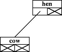The first argument of tree/3 will be the element in the node, and the second and third ones will be the left and right subtrees, respectively. Thus, an expression like

tree(hen, tree(cow, void, void), void)

represents the tree depicted in Figure 3.4.

  

Figure 3.4: A tree

As we did with lists, we can write a predicate which is true if its argument is a tree, as we have agreed to represent it; we do not pay any attention the the elements actually stored in the tree:

is_tree(void).
is_tree(tree(Info, Left, Right):-
   is_tree(Left),
   is_tree(Right).

Checking whether an element is stored or not in a tree is slightly more involved than in the case of the lists, since that element might be present in any of the two subtrees: different clauses are used for elements present in the root of the tree, in the left child, or in the right child:

tree_member(Element, tree(Element, L, R)).
tree_member(Element, tree(E, L, R)):- tree_member(Element, L).
tree_member(Element, tree(E, L, R)):- tree_member(Element, R).

Note that there is no clause for the case of a void tree: if the tree is void, then the call to the predicate must fail, because there is no information in it. Not having a case for a void tree makes the call fail in this case.

Updating a tree is also an interesting task: we want to define a predicate update_tree(OldElem, NewElem, OldTree, NewTree), whose meaning is quite obvious. The implementation resembles the code for tree_member/2:

update_tree(Old, New, tree(Old, R, L), tree(New, R, L)).
update_tree(Old, New, tree(Other, R, L), tree(Other, NR, L)):-
   update_tree(Old, New, R, NR).
update_tree(Old, New, tree(Other, R, L), tree(Other, R, NL)):-
   update_tree(Old, New, L, NL).

Trees can be traversed, and the contents of their nodes stored in lists. We give below a predicate which relates a tree with a list which stores the items in this tree in the order in which they are found when the tree is traversed in preorder (root first, then left child, then right child):

pre_order(void, []).
pre_order(tree(X, Left, Right), [X|Order]):-
   pre_order(Left, OrdLft),
   pre_order(Right, OrdRght),
   append(OrdLft, OrdRght, Order).

Problem 3.19   Define, similarly to the example before,

    in_order(Tree, Order) 
    post_order(Tree, Order)

$\blacklozenge$

Problem 3.20   Make versions of the predicates in Problem 3.19 using Prolog IV's o/3 constraint. $\blacklozenge$

$\mathbf\therefore$

One of the good things about binary trees is that if they are kept ordered, searching is relatively cheap. In a well-balanced binary tree, where an order relation is defined among the items it contains (suppose a precedes/2 predicate, as in the lists case), searching for an item can be made in $O(\log n)$, where n is the number of nodes in the tree. This search procedure can be implemented as follows:

search_ordtree(Element, tree(Element, L, R)).
search_ordtree(Element, tree(This, L, R)):-
   precedes(Element, This),
   search_ordtree(Element, L).
search_ordtree(Element, tree(This, L, R)):-
   precedes(This, Element),
   search_ordtree(Element, R).

We are assuming that items which precede a given element are stored in the left subtree. Conversely, the construction of the tree must respect this order, so, as it happened with lists, a new ordered tree cannot be built just by putting together two sons and a new piece of information: we want the resulting tree to be ordered, and without repetitions. The code for insert_ordtree(El, Tree, NewTree) is:

insert_ordtree(Element, void, tree(Element, void, void)).
insert_ordtree(Element, tree(Element, L, R), tree(Element, L, R)).
insert_ordtree(Element, tree(This, L, R), tree(This, NL, R)):-
   precedes(Element, This),
   insert_ordtree(Element, L, NL).
insert_ordtree(Element, tree(This, L, R), tree(This, N, NR)):-
   precedes(This, Element),
   insert_ordtree(Element, R, NR).